Making Sense of Attention
![]()
When it comes to deep learning few ideas have brought about such a radical shift in thinking as attention. Attention changed everything. Like other landmark ideas before it, attention draws merit from simplicity. In this post we’ll motivate attention as a natural way of looking at sequences and dig into three common attention mechanisms you’ll encounter in the wild.
Seq2seq#
Seq2seq makes use of two networks to transform one sequence into another. The first network, the encoder, represents the input sequence as a sequence of hidden states. The second network, the decoder, uses the final hidden state to generate an output sequence. By decoupling the input and output into two separate stages, seq2seq allows the ordering and length of the two sequences to differ, something an ordinary recurrent network cannot do. Attention was born out of an inherent limitation of the original seq2seq framing: a single vector bears responsibility for representing the entire input sequence.
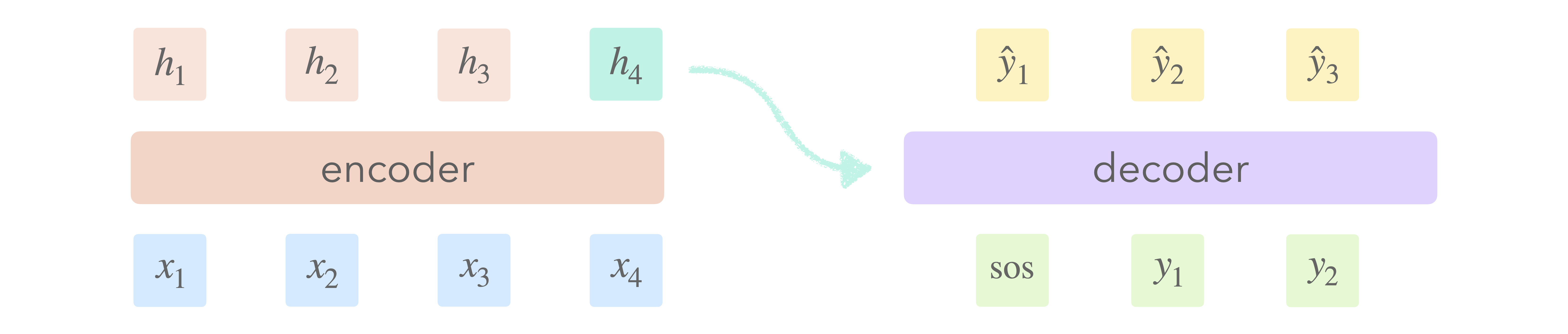
This bottleneck prevents the decoder from accessing (or more provacatively, querying) the full input sequence during the decoding process. After the final encoder state is passed to the decoder we no longer have access to the input sequence and must rely solely on memory. Not only does this make things more difficult, it’s tremendously wasteful, as we ignore all but the final encoder state.
The key insight of attention is that it would make life much easier if instead we could look at the entire input sequence while decoding. The question of how exactly we do that is where the fun starts. The sequence of encoder states is a learned representation of the input sequence. How can we utilize this sequence fully when decoding? One option is to simply pass the decoder the concatenation of all encoder states, however, this quickly leads to an explosion in the number of decoder parameters. Another option is to pass the decoder a weighted sum of encoder states and that’s exactly what attention does.
Seq2seq + Attention#
The basic setup of attention consists of four steps.
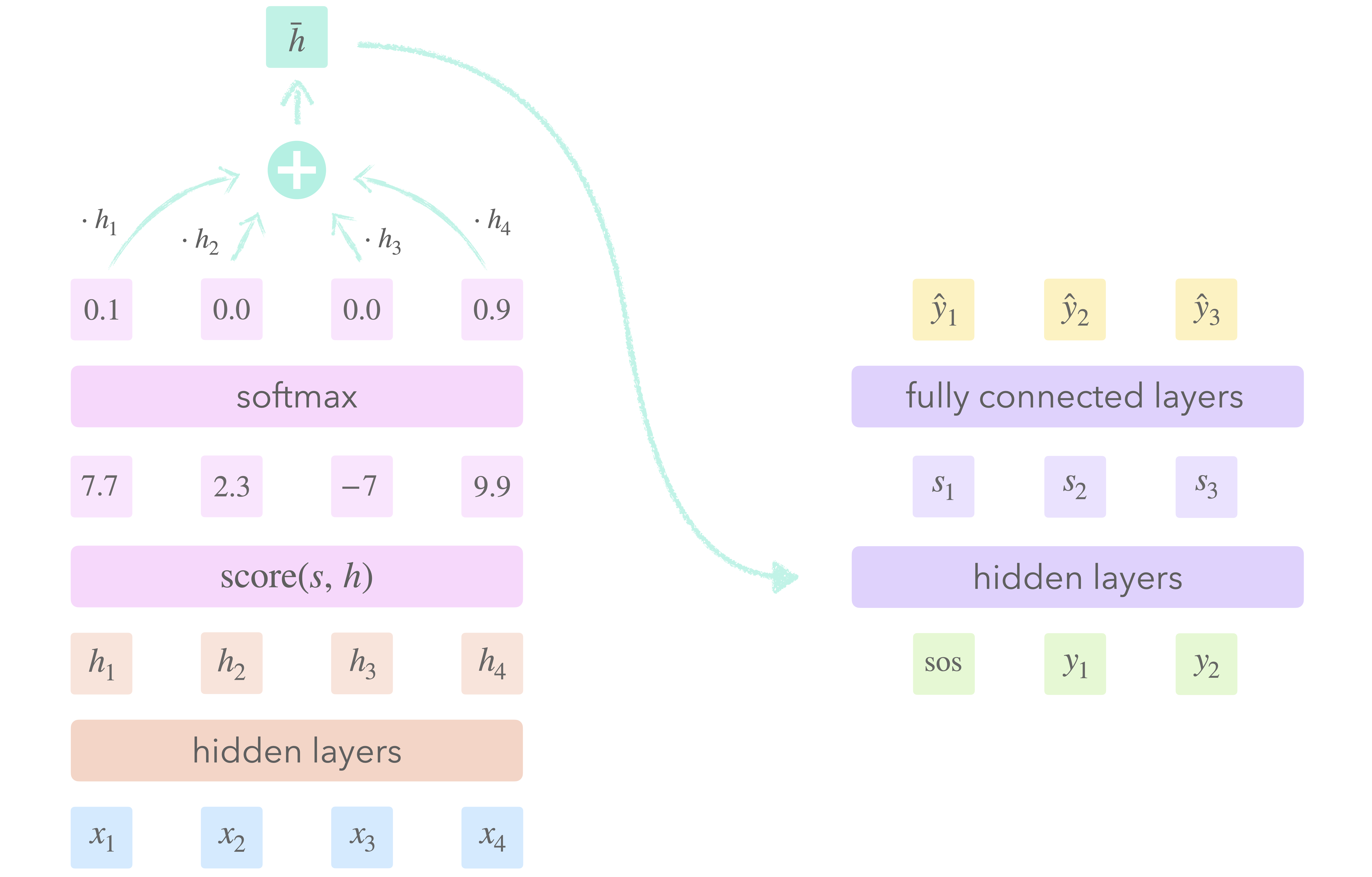
At each step of the decoding process, we
- Assign a weight to each encoder state $h$ of the input sequence: the attention score. This score depends only on $h$ and the current decoder state $s$.
- Normalize the attention scores to form a probability distribution.
- Sum the encoder states weighted by the attention scores to get a single vector: the context $\bar{h}$.
- Compute the next decoder state using the current context and decoder state.
Now, technically there is no requirement to turn the attention scores into a probability distribution before computing the context, however, there are at least two reasons we should. First, it aids interpretability by making it easy to see which inputs are relevant to the current output. Second, it ensures the expected value of the context vector is the same regardless of the length of the input sequence (in fact, the context has the same expected value as the individual encoder states). This matters since the context is passed through linear layers, which are sensitive to the magnitudes of their input on both the forward and backward pass (larger inputs produce larger gradients).
By providing the decoder a different context vector at each decoding step, attention allows the decoder to search through the input sequence for information relevant to the current output $y$. All we need to decide is how we’ll compute the attention scores themselves. Since we want to weight each input based on its relevance to $y$, it makes sense to look at which encoder states $h$ are close to the current decoder state $s$ in latent space. Mathematically speaking, there are many ways to define what “close” means, but none is simpler than the dot product.
Dot Product#
The dot product of two vectors is the product of their magnitudes scaled by the cosine of the angle between them.
\[ \mathbf{u} \cdot \mathbf{v} = \Vert \mathbf{u} \Vert \Vert \mathbf{v} \Vert \cos \theta \]
The dot product achieves its maximum when two vectors point in the same direction and its minimum when they point in opposite directions. The more similar two vectors are, the larger their dot product; the more dissimilar they are, the more negative their dot product. Two vectors that are independent of each other have a dot product of zero.
These three states make attention intuitive. Imagine we’re training an autoencoder on the sentence Helga ate an apple. The first word we must predict is Helga. Now the name Helga might conjure many connotations (honesty and the color yellow, for example), but presumably none of them have much to do with the words ate, an, and apple. Were every word to have a magnitude of one, we’d expect the dot product of Helga with each word to be

Applying softmax to these scores yields the final attention weights.

As we’d expect, Helga is weighted the highest, but what’s more interesting is how small the gap with the other weights is. Were Helga to have a magnitude of two the attention scores would be

and the attention weights would be

When every vector has a magnitude of one, the dot product is the same as cosine similarity. Because cosine similarity ignores magnitudes, it effectively confines each vector to the unit sphere. Since there’s not as much room to run around on the sphere as there is in general $d$-dimensional space, the values produced by cosine similarity have less variance, which yields a smoother softmax distribution. In this sense cosine similarity acts as a regularizer. Perhaps this is one reason to prefer the dot product, as it’d make more sense for the final weights to be skewed more towards Helga.
Scaled Dot Product#
There’s just one problem: the dot product tends to produce larger values in higher dimensional space (where distances can be larger), which saturates the softmax function and yields smaller gradients, making training more difficult. To avoid this, we need to normalize the dot product in such a way that the magnitude of its output is independent of the hidden dimension $d$. The only question is what we should divide by.
\[ \mathrm{score}(\mathbf{u}, \mathbf{v}) = \mathbf{u} \cdot \mathbf{v} \; / \; \mathbf{?} \]
Our first thought might be to simply divide by $d$ and that’s a good guess, but we can do something slightly more sophisticated. Let’s assume the components of a hidden state are independent random variables drawn from a standard normal distribution.
\[ \mathbf{u} = [u_1, \; \dots, \; u_d] \qquad u_i \sim N(0, 1) \]
We’ll show the dot product of two such hidden states has a mean of $0$ and a variance of $d$, hence dividing by $\sqrt{d}$ scales the variance to $1$, which leaves us free to choose the hidden dimension without affecting the magnitude of the attention scores. Were we to instead divide by $d$, the resulting variance would be $1/d$, meaning the attention scores would be more similar the larger $d$ is (in the limit all scores converge to zero, which yields a uniform softmax distribution and completely negates the effect of attention).
Working this out is a fun exercise and makes things more concrete. To start,
\[ \mathbf{u} \cdot \mathbf{v} = u_1v_1 + \cdots + u_dv_d \]
If we can show the products $u_i v_i$ are independent and of unit variance, we’re done, since the variance of the sum of indepedent random variables is the sum of their variances.
\[ \mathrm{Var}(u \cdot v) = \mathrm{Var}(u_1v_1) + \cdots + \mathrm{Var}(u_dv_d) = d \]
First, independence. The $i$-th component of each hidden state represents an independent random variable $X_i$, hence the products $u_i v_i$ and $u_j v_j$ represent random variables $X_i^2$ and $X_j^2$. The only question is whether they’re independent or not. It’s a very nice fact that applying a “nice” function to a collection of independent variables preserves independence. Since the square is indeed a nice function, this fact tells us that $X_i^2$ and $X_j^2$ are also independent.
Showing that the product of two independent random variables $X_i, X_j \sim N(0, 1)$ has unit variance is just a matter of applying the right identities.
\begin{align} \mathrm{Var}(X_iX_j) &= \mathrm{E}[X_i^2X_j^2] - \mathrm{E}[X_iX_j]^2 \\ &= \mathrm{E}[X_i^2X_j^2] - \mathrm{E}[X_i]^2\mathrm{E}[X_j]^2 \\ &= \mathrm{E}[X_i^2]\mathrm{E}[X_j^2] \\ &= 1 \end{align}
The first equality follows from the definition of variance, the second from the independence of $X_i, X_j$, and the third from the independence of $X_i^2, X_j^2$ and the fact that $X_i, X_j$ have zero mean. The last equality follows from the easy fact that the square of a standard normal has a mean of one.
\[ 1 = \mathrm{Var}(X) = \mathrm{E}[X^2] - \mathrm{E}[X]^2 = \mathrm{E}[X^2] \]
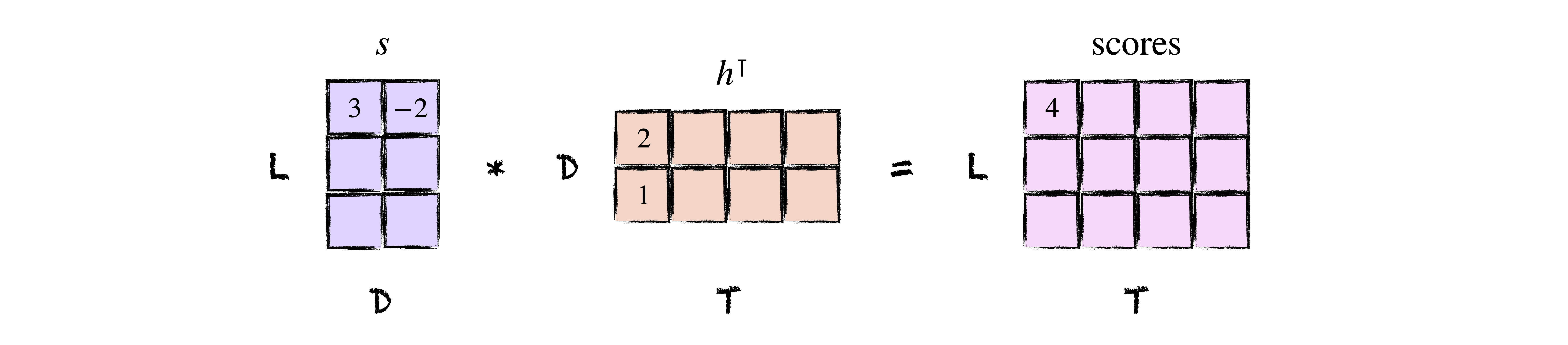
Neat, right? The last thing to do is to express things in code. As usual, the only thing we really need to be mindful of are the shapes. An input sequence of length $T$ yields a matrix of encoder states $h$ of shape $(T, D)$ and a matrix of decoder states $s$ of shape $(L, D)$. To take the dot product of each encoder state with each decoder state, we can simply multiply $s$ and $h^\intercal$ to get a matrix of scores of shape $(L, T)$ whose $ij$-th entry is the dot product of $s_i$ and $h_j$. How cool is that?
class DotScore(nn.Module):
    """Scaled dot product as an attention scoring function."""

    def __init__(self, d: int):
        super().__init__()
        self.d = d

    def forward(self, s: Tensor, h: Tensor) -> Tensor:
        # (B, L, D) x (B, D, T) -> (B, L, T)
        return s @ h.transpose(1, 2) / math.sqrt(self.d)
Treating the length $L$ of the target sequence as a variable allows our code to handle both the case when we have just one decoder state available at a time (e.g. when using a recurrent network) and the case when we have all decoder states available at once (e.g. when using a transformer).
A Generalized Dot Product#
As we mentioned earlier, there are many ways to define what it means for two vectors to be close. The dot product is the most natural way, but it is not the only one. Mathematically speaking, a notion of closeness comes from an inner product, which you can think of as nothing more than a generalized dot product. More specifically, an inner product is a bilinear map with some nice properties that takes two vectors as input and outputs a number.
\[ \langle\mathbf{u}, \mathbf{v}\rangle \; \longmapsto \; \mathbb{R} \]
Sounds suspiciously like a way to measure distance, doesn’t it? Choosing a basis allows an inner product to be represented as a matrix $\mathrm{W}$.
\[ \langle \mathbf{u}, \mathbf{v} \rangle = \mathbf{u} \mathrm{W} \mathbf{v}^\intercal \]
For example, the dot product over $\mathbb{R}^2$ with the usual basis is represented by the identity matrix.
\[ \mathbf{u} \cdot \mathbf{v} = \begin{bmatrix} u_1 & u_2 \end{bmatrix} \begin{bmatrix} 1 & 0 \\ 0 & 1 \end{bmatrix} \begin{bmatrix} v_1 \\ v_2 \end{bmatrix} = u_1v_1 + u_2v_2 \]
More generally, an inner product over $\mathbb{R}^2$ is represented by a matrix
\[ \mathrm{W} = \begin{bmatrix} a & b \\ b & d \end{bmatrix} \quad \text{where} \quad \mathbf{u} \mathrm{W} \mathbf{u}^\intercal > 0 \;\; \forall \;\; \mathbf{u} \neq 0 \]
Choosing the dot product as the scoring function essentially hardcodes the values of this matrix. As machine learning enthusiasts, this feels a bit unnatural. Why not just learn the values of $a$, $b$, and $d$ instead? So-called “multiplicative” attention does just that and more: it ditches the constraint on $\mathrm{W}$ completely, allowing us to learn a general matrix
\[ \mathrm{W} = \begin{bmatrix} a & b \\ c & d \end{bmatrix} \]
and the associated scoring function
\[ \text{score}(\mathbf{u}, \mathbf{v}) = \mathbf{u} \mathrm{W} \mathbf{v}^\intercal \]
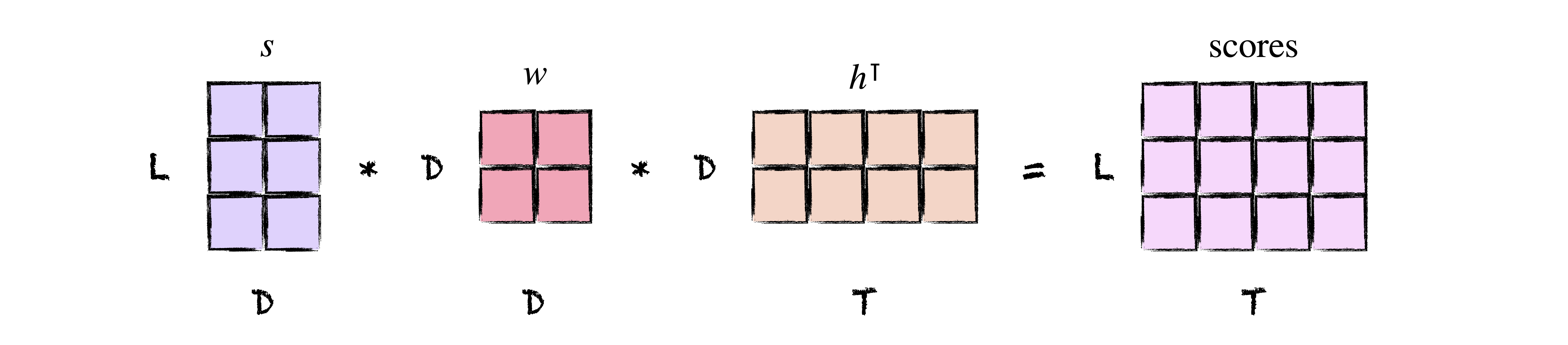
which may no longer be an inner product. Whereas the dot product weights each dimension equally, the above matrix can learn to weight each dimension according to its importance, allowing us to ignore insignificant parts of the latent space. Given that the latent space typically has hundreds of dimensions, we can expect some of them to be less informative than others.
At this point you might be wondering why we would ever choose the dot product as our scoring function when the above form can learn any bilinear map, including the dot product. Well, much as skip connections arose from the intuition that it’s harder to learn the identity mapping than the zero mapping, it can be difficult for the general form to converge to the dot product.
Implementing the above scoring function, which we’ll call the bilinear score, requires only a weight matrix of shape $(D, D)$.
class BilinearScore(nn.Module):
    """A generalized, trainable dot product as an attention scoring function."""

    def __init__(self, d: int):
        super().__init__()
        self.w = nn.Linear(d, d, bias=False)

    def forward(self, s: Tensor, h: Tensor) -> Tensor:
        # (B, L, D) x (D, D) x (B, D, T) -> (B, L, T)
        return s @ self.w @ h.transpose(1, 2)
Note that we can and should divide the output of the bilinear score by $\sqrt{d}\,$ for the same reason as with the dot product (the resulting variance may no longer be $1$ but will still be a constant), however, historically it did not include any scaling initially.
Learning to Score#
The last of the scoring functions we’ll cover is the simplest and most general. Just as it felt a bit unnatural to hardcode the values of the earlier $2 \times 2$ matrix, it feels a bit unnatural to force the scoring function to resemble an inner product. Why not just learn an arbitrary scoring function with a shallow fully connected network?
Such a network might take as input the concatenation of an encoder state $h$ and decoder state $s.$ You’ll often see this written as:
\[ \text{score}(\mathbf{h}, \mathbf{s}) = \mathbf{v}^\intercal \tanh(\mathrm{W} [\mathbf{s}; \mathbf{h}]) \]
where the semicolon denotes concatenation and $\mathbf{v}^\intercal$ denotes the second linear layer of this two layer network, somewhat confusingly denoted as the transpose of a column vector (because it outputs a single number).
Originally, the encoder and decoder states were fed through seaprate linear layers and then summed together before being passed through the final layer, giving rise to the name “additive” attention.
\[ \text{score}(\mathbf{h}, \mathbf{s}) = \mathbf{v}^\intercal \tanh(\mathrm{W}\mathbf{s} + \mathrm{U}\mathbf{h}) \]
We’ll stick with the former incarnation, which is sometimes called the “concat” score, as it typically leads to better performance. We use $\tanh$ as the activation function so the output of our scoring function yields an even distribution of positive and negative scores.
Implementing the concat score requires a bit of yoga, as we need to concatenate each encoder state with each decoder state. We’ll do this by repeating each decoder state $T$ times and the matrix of decoder states $L$ times. Then we’ll concatenate the two together along the hidden dimension into a matrix of shape $(L*T, 2D)$ and reshape the output into a matrix of shape $(L, T)$.
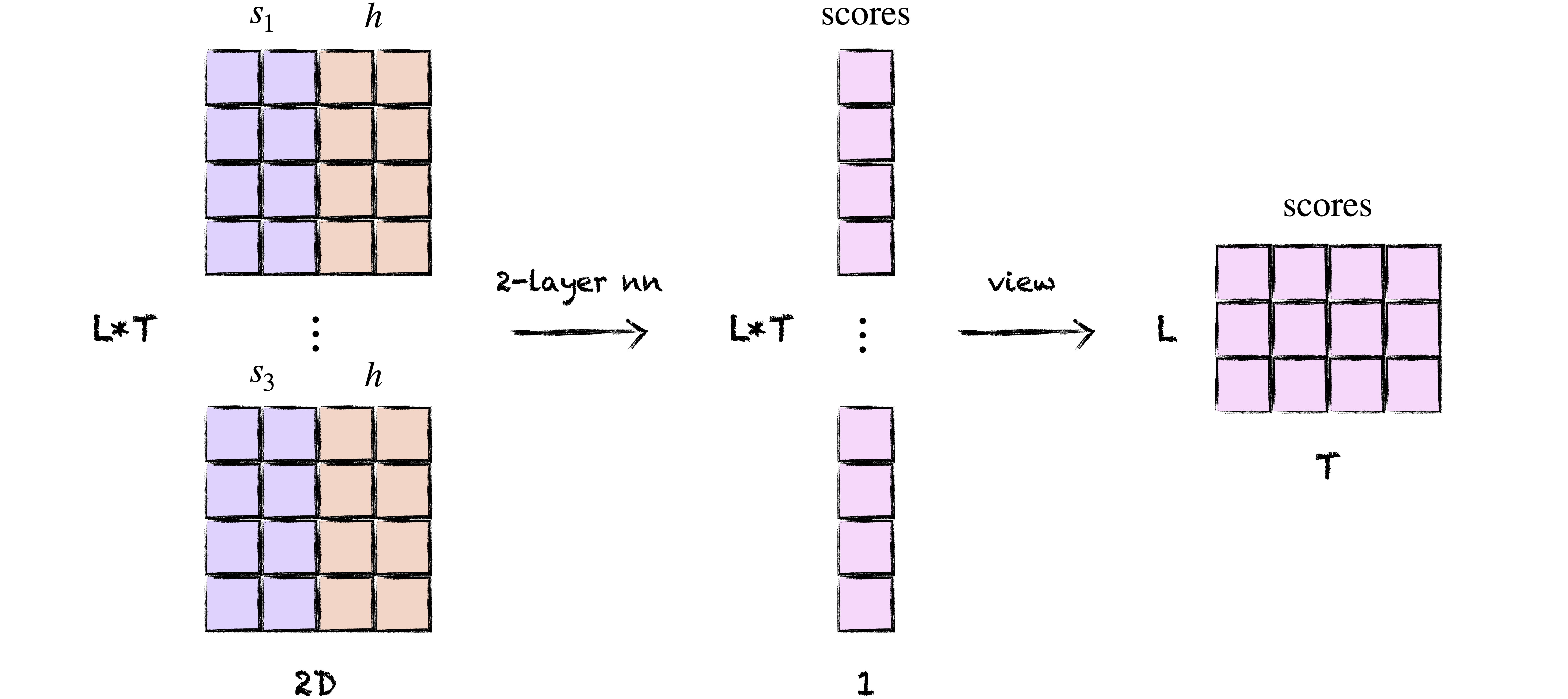
class ConcatScore(nn.Module):
    """A two layer network as an attention scoring function."""

    def __init__(self, d: int):
        super().__init__()
        self.w = nn.Linear(2*d, d)
        self.v = nn.Linear(d, 1, bias=False)

    def forward(self, s: Tensor, h: Tensor) -> Tensor:
        (B, L, D), (B, T, D) = s.shape, h.shape
        s = s.repeat_interleave(T, dim=1)                   # (B, L*T, D)
        h = h.repeat(1, L, 1)                               # (B, L*T, D)
        concatenated = torch.cat((s, h), dim=-1)            # (B, L*T, 2D)
        scores = self.v(torch.tanh(self.w(concatenated)))   # (B, L*T, 1)
        return scores.view(B, L, T)                         # (B, L, T)
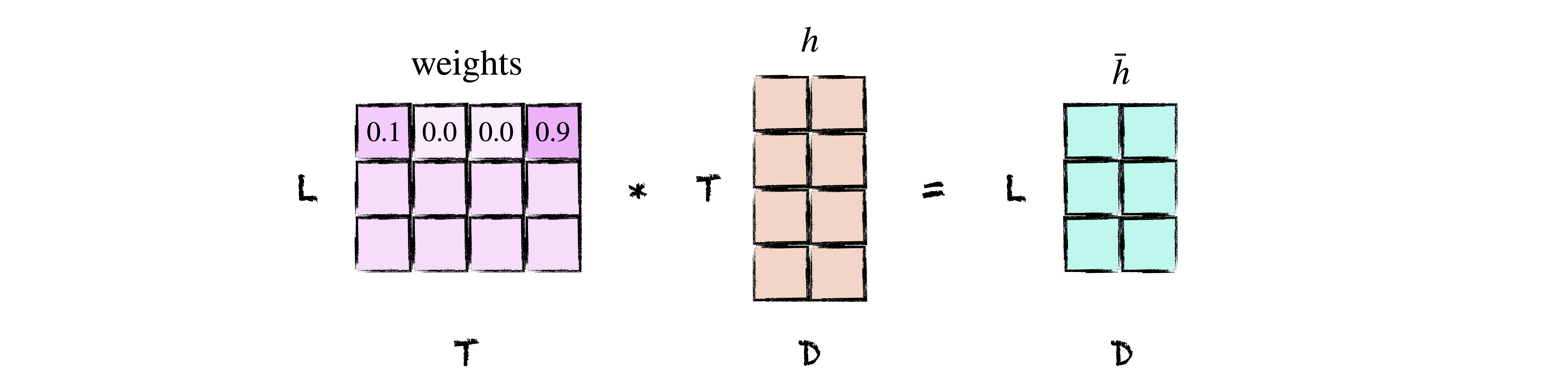
Computing the Context#
Once we have the raw attention scores the last thing to do is to normalize them and take a weighted sum of hidden states to get the final context vector $\bar{h}$. This is exactly what it sounds like with one twist: we’ll ignore padding in the input sequence by accepting a boolean mask that tells us which indices are padded so we can set the corresponding attention weights to zero. However, since setting the weights to zero directly invalidates the probability distribution, we’ll instead set the raw scores to a large negative number so that the resulting softmax weights are approximately zero. Since at inference time we typically do not pad inputs, our mask parameter will be optional.
class Attention(nn.Module):
    """Container for applying an attention scoring function."""

    def __init__(self, score: nn.Module):
        super().__init__()
        self.score = score

    def forward(self, s: Tensor, h: Tensor, mask: Tensor = None) -> Tensor:
        """Compute attention scores and return the context."""
        (B, L, D), (B, T, D) = s.shape, h.shape
        scores = self.score(s, h)                           # (B, L, T)
        if mask is not None:                                # (B, L, T)
            scores.masked_fill_(mask, -1e4)
        weights = F.softmax(scores, dim=-1)                 # (B, L, T)
        return weights @ h                                  # (B, L, D)
All Together Now: Query, Key, Value#
The below table summarizes each of the attention scoring functions we’ve covered today.
$\,$
| name | scoring function | source |
|---|---|---|
| dot product | $\mathrm{score}(\mathbf{s}, \mathbf{h}) = \mathbf{s} \cdot \mathbf{h}$ | Luong, 2015 |
| scaled dot product | $\mathrm{score}(\mathbf{s}, \mathbf{h}) = \mathbf{s} \cdot \mathbf{h} \;/\; \sqrt{d}$ | Vaswani, 2017 |
| bilinear (multiplicative) | $\mathrm{score}(\mathbf{s}, \mathbf{h}) = \mathbf{s} \mathrm{W} \mathbf{h}^\intercal$ | Luong, 2015 |
| concat (additive) | $\mathrm{score}(\mathbf{s}, \mathbf{h}) = \mathbf{v}^\intercal \tanh(\mathrm{W} [\mathbf{s}; \mathbf{h}]) $ | Bahdanau, 2015 |
We’ve learned that attention alleviates the information bottleneck of the original seq2seq framing by allowing us to look at the entire input sequence during the decoding process, and that it encodes a prior belief that the importance of each input is relative to what we are trying to predict. The entire process of attention can be captured in a single picture.
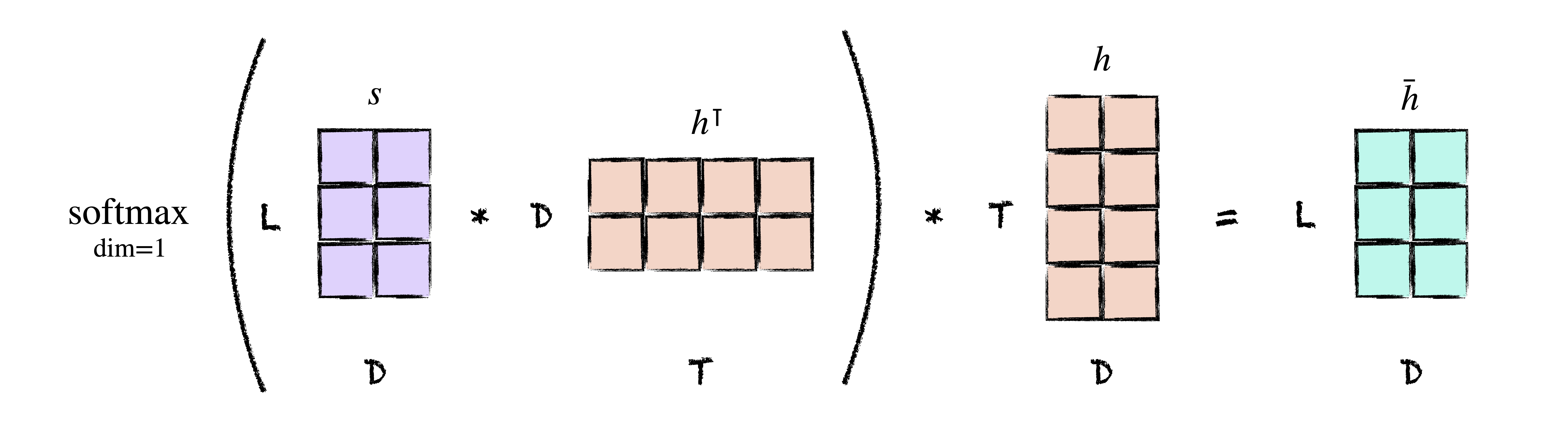
Of course, this picture is better known by what is likely the most famous equation in all of deep learning:
\[ \mathrm{Attention}(\mathrm{Q, K, V}) = \mathrm{softmax}\left(\frac{\mathrm{Q}\mathrm{K}^\intercal}{\sqrt{d}}\right)\mathrm{V} \]
where $\mathrm{Q}, \mathrm{K}, \mathrm{V}$ are so-called query, key, and value matrices. In our case, the decoder states $s$ are the queries and the encoder states $h$ are both the keys and values. Each decoder state represents a question (query): what inputs are relevant to the current output? Each encoder state represents a possible answer (key). Together, query and key assign a weight to the values we care about (the encoder states themselves).